The Anvikshik

Mapping of object oriented classes to relational tables

March 14, 2024

If you are a software engineer, then you would probably have gone through low-level design (LLD) interviews where you are asked to design the low-level components of a system and model the databases and APIs for it.
For example, designing a stackoverflow system is a common (LLD) question.





However, have you felt that once you got the class design figured out, creating relational tables is not an easy task. There is something that does not feel right.
For instance, say a User can vote(upvote/downvote) a Question and this has M:N relationship i.e 1 user can vote many questions and one question can be voted by many users. How would you model this as relational tables?


Would you create one 'User' table and add 'question_vote' as a column in it and then add a json string as value: "{ "question_id1": "upvote", "question_id2": "downvote", "question_id3": "none"} , ... }" ? But then querying this table to check if the current user has voted the current question would require loading up entire json string and parsing it.

Another option would be to have multi-valued attributes but that would mean denormalized database which makes querying much harder. What is the going on here ???

This issue that we are facing is called impedance mismatch. A term borrowed from electrical engineering, imepedance mismatch means that the two components of system have different structure and thus cannot seamlessely integrate with each other. In this OOD to relational mapping, this happens because both paradigms are based on different principles. OO design is based on software engineering principles while Relational design is based on mathematical principles. Thus we would need a way to map components from one paradigm to another. Let's see how we can do this component by component. Let's take the simple UML diagram as shown under:


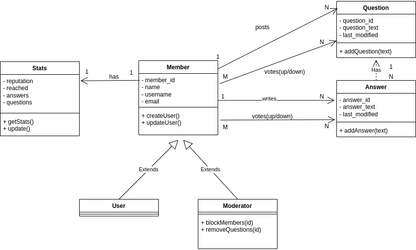
How to map classes
Classes can be mapped directly to tables with attributes being mapped to columns. For e.g. table for Member would look something like this:
Member
-------------------------------------------------------------
member_id | name | username | email | image | ...


How to map inheritance i.e "is-a" relationship
There are actually three ways we could model the inheritance relationship.
1. Map entire hierarchy to one table
We can map the entire hierarchy to one table and the individual types can be modeled as types. For e.g, the Member hierarchy can be modeled as:
Member
-------------------------------------------------------------
member_id | name | username | email | image | member_type_id
-------------------------------------------------------------
1 | John | john23 | john@gmail.com | 'default.jpg' | 2


Member_type
-------------------------------------------------------------
type_id | type_name
-------------------------------------------------------------
1 | User
2 | Moderator


The advantage of this approach is that it is easy to implement and very easy to add new types. Say, if we have an 'admin' type tomorrow, then we can add a new type in Member_type table and just start using it.
The disadvantage is that classes are highly coupled. This means that changing/adding attributes in one class affects another. For e.g if we want 'moderators' to have 'payment_id' attribute then we need to add this to Member table. But this would expose it to 'users' as well who should not know about it. Thus we are voilating the "principle of least priviledge" .


2. Map each concrete class to its own table
We can create tables for each concrete class. For e.g. we can have following tables in DB:
User
-------------------------------------------------------------
user_id | name | username | email | image
-------------------------------------------------------------
1 | John | john23 | john@gmail.com | 'default.jpg'


Moderator
-------------------------------------------------------------
moderator_id | name | username | email | image
-------------------------------------------------------------
1 | Alice | alice1 | alice@gmail.com | 'default.jpg'


The advantage of this approach is that all data of a class is stored at one place thus making reads/writes faster.
The disadvantage is that if an attribute is changed in base class, then we need to update the same in derived classes as well.


3. Map each class to its own table
We can create one table for each class. For e.g we can have following tables in DB:
Member
-------------------------------------------------------------
member_id(PK) | name | username | email | image
-------------------------------------------------------------
1 | John | john23 | john@gmail.com | 'default.jpg'
2 | Alice | alice1 | alice@gmail.com | 'default.jpg'


User
-------------------------------------------------------------
member_id(FK) | user_specific_attrs
-------------------------------------------------------------
1 | ...


Moderator
-------------------------------------------------------------
member_id(FK) |moderator_specific_attrs
-------------------------------------------------------------
2 | ...


The advantage of this approach is that we don't need to update derived class table if there is change in base class table. Another advantage is that there can be overlapping roles i.e same user can also be a moderator. This was not handled in previous two approaches.
The disadvantage is that data is now distributed. Need to make joins to collect information for same user.


How to map relationships (1:1, 1:N, M:N)
Mapping 1:1 relationship
Mapping 1:1 relationship is the simplest as we can simply use the primary_key of one table as the foreign key in another.
For instance, in the Stats table, we can use member_id as the foreign key, thus linking a user to its stat. We could done the other way as well i.e have a stats_id as foreign key in the Member table.

Mapping 1:N relationship We can use the foreign key in the table where we can have only 1 instance of the other. For e.g. 1 question can have many answers but 1 answer is associated with only 1 question. Thus, it makes sense to have 'question_id' as the foreign key in the Answer table.

Mapping M:N relationship The best approach to map a many-to-many relationship is to use an associative table which uses the primary keys of both the tables. For e.g, we can create a table called 'MemberQuestion' which contains member_id, question_id and vote as the columns. This way we can find all the questions voted by a given member and how many votes has been received by a given question.

MemberQuestion
-------------------------------------------------------------
member_id(FK) |question_id(FK) | vote
-------------------------------------------------------------
1 | 1 | upvote

Inference of llama2 on 4GB GPU

December 18, 2023

Large language models such as llama2 has parameter size ranging from 7 Billion to 70 Billion. These models require large amount of GPU memory for inference. According to Nvidia :

Turns out that we can. Let's see how we can do this.

Layer-wise inference


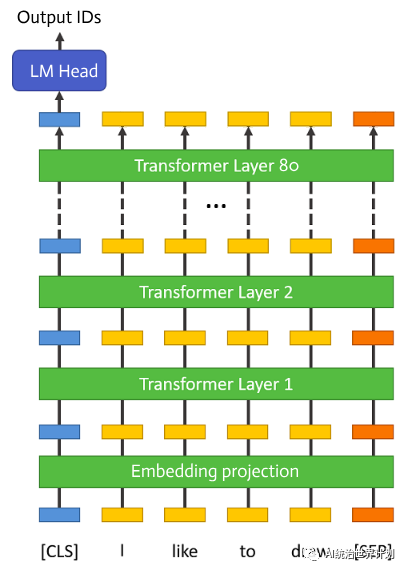
The large language models have around 32 to 80 identical layers after the embedding layer. Each layer is used sequentially for inference i.e ouput of one layer is fed as an input to next layer.
If we can load one layer in GPU at a time, saving the output in RAM temporarily, we would be consuming around 1/n of original space where n is the memory needed for n layers. Thus GPU memory required per layer would be 30GB/32 = 0.9 GB. This is the main idea behind how we can reduce the memory footprint. The other way is to use quantization. In fact, we can use both the approaches. Is there a library to do this ? Yes, we can use AIRLLM.

How to use the airllm package?

pip install airllm
Code:

                                
from airllm import AirLLMLlama2
MAX_LENGTH = 128
local_model = "/home/user/.cache/huggingface/hub/models--meta-llama--Llama-2-7b-chat-hf/snapshots/c1b0db933684edbfe29a06fa47eb19cc48025e93"
model = AirLLMLlama2(local_model,compression='4bit')
input_text = [
    'how to transition from swe to ml roles',
]

input_tokens = model.tokenizer(input_text,
    return_tensors="pt", 
    return_attention_mask=False, 
    truncation=True, 
    max_length=MAX_LENGTH, 
    padding=True)

generation_output = model.generate(
    input_tokens['input_ids'].cuda(), 
    max_new_tokens=1000,
    use_cache=True,
    return_dict_in_generate=True)

output = model.tokenizer.decode(generation_output.sequences[0])

print(output)
                                
                                

Obstacle Avoiding Robot

February 16, 2022

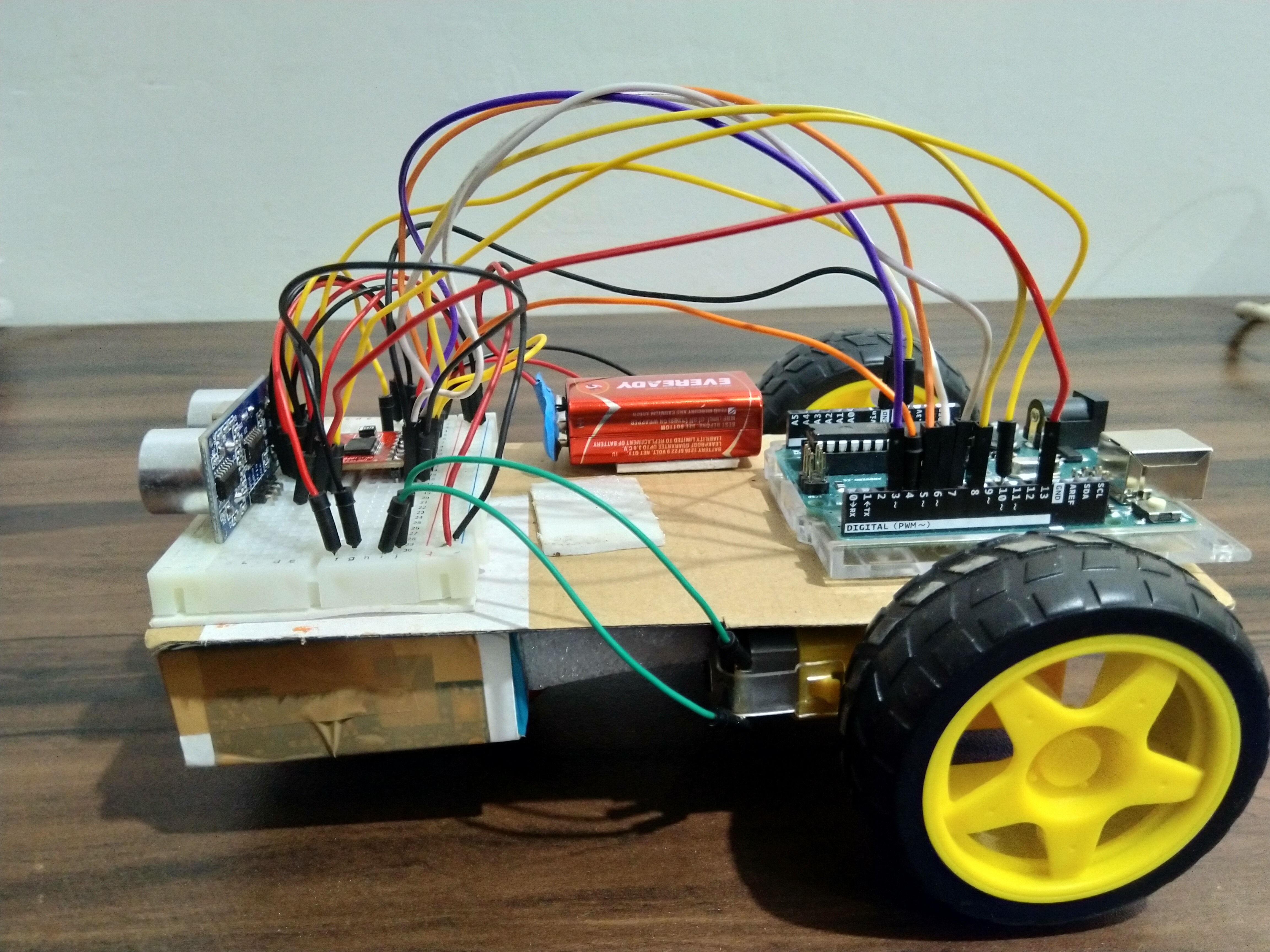
Obstacle avoiding robot is a robot that could move around freely by avoiding the obstacles. There are a lot of tutorials on the internet that you could lookup to create one yourself. However, If I had to recommend, I would say dronebotworkshop is one of the best. The main reason I have created this post is to share the mistakes I did so that you don't repeat it. Let's start.

• Mistake 1: Servo motors vs DC motors
I thought initally both are motors and could be used interchangeably but I was wrong. Servo motors are precision-based motors that don't rotate more than 180 degress and are used as robotic limbs, rudder control or for car-wiper kind of movement. Although you can do some adjustments (like removing potentiometer) to create a continuous rotating servo motors but it is very hard. Also, it is hard to find continuous rotating servo motors.

DC motors or battery-operated DC motors, on the other hand, can rotate continuosly and are used as wheels of cars etc.
There are another kind of motors called Stepper motors that are like fine-tuned servo motors and are used for 3d printer kind of situations.

So use a battery operated DC motors for a robot that needs to rotate continuosly. I used DC motors with voltage range 3~6 V. Remember more the volatage required for a motor, more the voltage is needed in a battery.


• Mistake 2: L298N module vs TB6612FNG module
There are a lot of tutorials with L298N module and it's very easily available as well. Initially, I used L298N module to drive the motors. It was working great but after some time the motors would start to slow down and eventually stop. There was only some noise but motors wouldn't work. Replaced it with new battery and same thing happened again. I did a digup on the internet and found that L298N module has very poor efficieny(around 45%) and it is dropping the voltage really quick. So as a hack, I powered the logic with arduino's 5v but still it wouldn't work for long.

I searched and found about another H bridge circuit-TB6612FNG. It's a really awesome module and I would advise you to use it rather than L298N module. It has very high efficieny(around 95%) and it can provide constant volatage/current to the motors.


• Mistake 3: Not soldering module
The TB6612FNG module comes with male header pins that are not soldered. I thought I could insert it into breadboard using the pins and it should work. But it didn't. So I had to solder it to make it work. I guess this was a silly mistake when I look back. But then that's the part of learning.

Boolean Retrieval

August 05, 2020

Suppose we want to find which plays of Shakespeare from Shakespeare's Collected Works, contain the words Brutus AND Caesar AND NOT Calpurnia. There are multiple ways to do it. One way is to search every document(using computers) and note down which documents contains Brutus and Caesar but not Calpurnia. 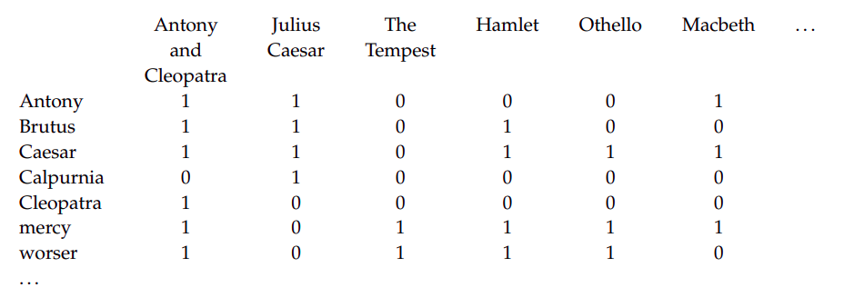Fig1. A term-document incidence matrix

Another way is to index the documents in advance and create a matrix as shown in the Fig 1. where for each play(column) we mark the cells 1 if it contains the word(row). It is also called term-document incidence matrix.

To answer the query: Brutus AND Caesar AND NOT Calpurnia, we take vectors of the first two terms and AND it with the complement of the last term i.e. 110100 and 110111 and 101111 = 100100 . Thus, the answer is Antony and Cleopatra and Hamlet. Since this model contains 0 and 1 for occurence or abscene of a word, it is called Boolean retrieval. The problem with the above solution is that the matrix becomes too big for computer's memory for large corpus of documents containing distinct terms.

If we look closely ... we find that the matrix is sparse i.e only a small subset of words are present in a document. Thus an effective way to store the presence of words in documents is to record only 1s and create an inverted index. 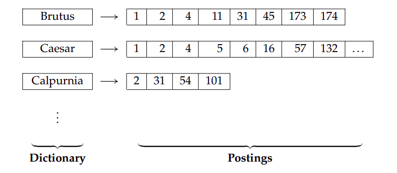Fig2. An inverted index with a collection of words on left side(called dictionary) and a list of documents in which the term occurs(called postings).

Fig2. shows an inverted index for the terms made by creating a list of the documents in which the term occurs. Now for the query: Brutus AND Caesar AND NOT Calpurnia, we locate Brutus, Caesar, and Calpurnia and retrieve their postings and find the intersection between first two and then remove the words that is present in Calpurnia. That is from the intersection of postings of Brutus and Caesar we get 1,2,4. If we remove 4 from it, we get the result as 1,2 which is Antony and Cleopatra and Hamlet.

Often on Leetcode and other sites, we find problems such as intersection of two lists or k lists. This is a perfect instance where rubber meets the road. For e.g. if you have two sorted lists of roughly equal size and want to find the common elements between them, the best approach woulld be to use two pointers. But if one of them is very large, then it would make more sense to apply binary search for the elements present in shorter list.

Now if you have multiple lists of varying size then you can either sort them and start by finding common with the two smallest lists and then its result with next smallest and so on, or you can handle two lists at a time and form a hierarchical way to find the intersection. The best approach usually is the one which tends to be most simple and handles the constraints well.

References- Manning, Raghavan, Schultze
Image Credits- shakespeare birthplace trust

TF-IDF

August 20, 2020

In the previous post, we saw that intersection of postings resulted in list of common postings for the query. Does it matter in which order should we show the result to the user? It turns out that it does matter.

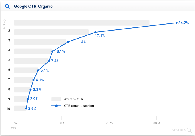Fig1. Ranking of webpages vs CTR

We can see in the figure 1 that the site that is ranked 1 has CTR (click-through rate) of 34% while the next site that is ranked 2 has CTR of 17%. This exponential decrease shows that 60% people tend to find their information need satisfied from first three sites. In another study it has been found that the order of relevance matter i.e if the ranked 1 site(most relevant) is swapped with ranked 2 site(less relevant), then CTR of rank2 increases. Hence it is important to factor in the ranks when retrieving the documents for a given query.

The next logical step to rank two or more documents for a free-form query such as we type in search engines (as opposed to the boolean query of last post) is to find the number of occurences of the query term t in the document d. To calculate the score/rank ... we find the frequency of all terms of query in the documents, sum them up and rank them in decreasing order. This weighting is called term frequency. 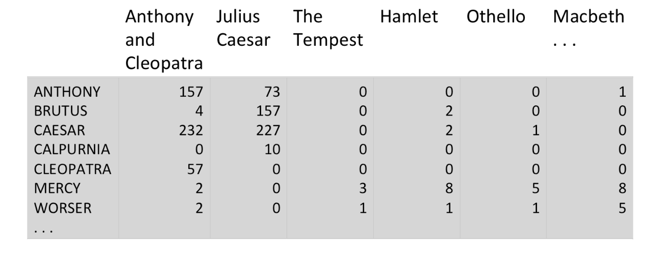Fig2. Frequency of the terms in the documents

Figure 2 shows the number of occurences of the terms (raw term frequency) in the documents. But the raw term frequency has problem that relevancy does not increase with term frequency i.e. a document with tf=10 is more relevant than a document with tf=1 but not 10 times more relevant. Thus we can solve this problem by taking logarithm of tf for term t in document d: $$w_{t,d}= 1+log_{10}tf$$ Another problem is that all terms are considered equally important when assessing the relevancy. However, this is not true. For instance in a set of documents from law industry, the term legal will be in almost all the documents. So we need to attenuate the occurence of frequent terms and increase weight for rare terms. This can be done by using document frequency which is defined as the number of documents that contain the term t. To weight tf we will use inverse document frequency which is defined as: $$ idf_t= \log_{10} \frac{N}{df_t} $$ where N is the number of documents in the collection. This brings us an important milestone in IR which is tf-idf weighting and defined as: $$ w_{t,d}= (1+log_{10}tf) * \log_{10} \frac{N}{df_t} $$ tf-idf weight increses with the number of occurences within a document(term-frequency) and increases with the rarity of the term in the collection (inverse document frequency). 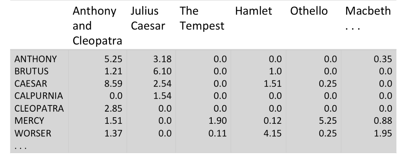Fig3. tf-idf weights for the terms in the documents

For our initial query of:Brutus and Caesar but not Calpurnia, the score for Anthony and Cleopatra will be 1.21 + 8.59=9.80 while the score for Hamlet will be 1.0+1.51=2.51. Thus,Anthony and Cleopatra is more relevant for the query and should be displayed above Hamlet.

Image Credits for ranking- Sistrix
Image Credits for shakespeare term matrix- Prof. Cav

Vector Space

August 21, 2020

In the last post, we saw how to calculate the tf-idf weights for the terms the documents. Today, we will see how we can use it in a different way.

Gerald Salton, the father of information retrieval introduced the concept of vector space where each document can be treated as a vector of tf-idf weights \( \in R^{|V|} \) thus leading to a |V| dimensional real-valued vector space. Then terms can be treated as axes and documents as vector in this vector space. 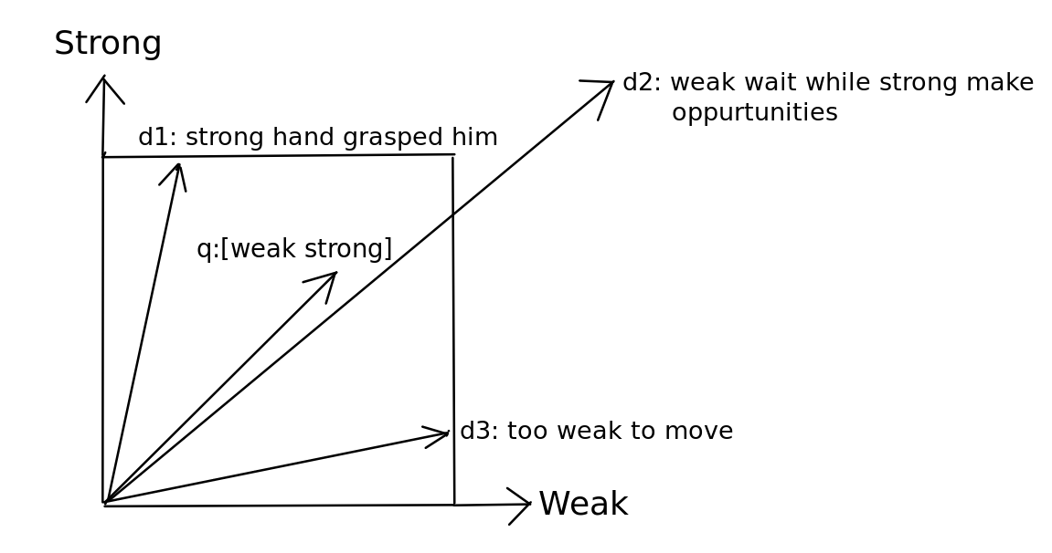Fig1. Vector space where terms are axes, while query and documents are vectors

For example, in the figure 1, we can suppose the terms Weak and Strong to be the two axes- x and y respectively. Since the document \(d_1\) is semantically related to Strong, vector of \(d_1\) will be closer to y axis, while the document \(d_3\) is semantically related to Weak, vector of \(d_3\) will be closer to x-axis.

On the other hand, \(d_2\) contains references to both Weak and Strong and thus it's vector will be in the middle. For the query: weak strong, which could be also be represented as vector (consider it as short document), we find that its vector is near the vector of \(d_2\) as it contains references to both Weak and Strong.

Now, we can rank the documents based on the similarity or proximity of the query vector with the vector of the documents. The question is how do we find the similarity of two vectors?

Euclidean distance is not a good option since ... we can see in the figure itself that distance between q and \(d_2\) is larger compared to distance between q and \(d_1\), although q is semantically closer to \(d_2\). Angle betweent the vectors will be a good idea. The smaller the angle the better the similarity. In fact, we can use the cosine of the angles since cosine of two vectors is their dot product if they are length normalized. We need length normalization to account for documents that are similar but have different lengths.
$$ cos(q,d)= \frac{\Sigma_{i=1}^{|V|} q_i d_i}{\sqrt{\Sigma_{i=1}^{|V|} q_{i}^{2}} \sqrt{\Sigma_{i=1}^{|V|} d_{i}^{2}}}$$ where \(q_i\) is tf-idf weight of term i in the query and \(d_i\) is tf-idf weight of term i in the document. The denominator represents that query and documents are normalized.

Let's take an example to understand how cosine is calculated. Assume that we have three novels- Austen's Sense and Sensibility , Pride and Prejudice and Bronte's Wuthering Heights. We take three terms with normalized log term frequency (we don't do idf-weighting to keep it simple) as shown in the figure 2. 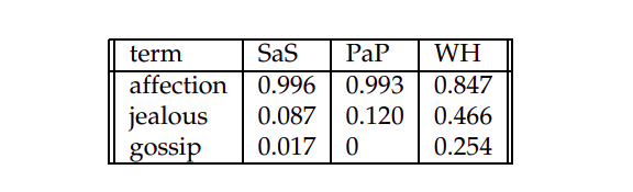Fig2. Normalized log term-frequency weights of SaS,PaP,and WH

Then,
\(cos(SaS, Pap) = 0.996 * 0.993 + \) \(0.087 * 0.120 + 0 = 0.999 \)
\(cos(SaS, WH) = 0.996 * 0.847 + \) \(0.087 * 0.466 + 0.017 *0.254 = 0.888\)
\(cos(PaP, WH) = 0.993 * 0.847 + \) \(0.120 * 0.466 + 0 = 0.896\)

It can be seen that cos(SaS, PaP) is greater than other two which is obvious since SaS and PaP are both written by Austen.

One important thing we can learn from vector space is how to turn the simple matrix of numbers into a n-dimensional space. An example of this concept would be the word embeddings- where we turn or map words to a bunch of real numbers (Tomas Mikolov, 2013) and words that are alike are nearby while words that are different are far away in this n-dimensional space.

Tutorial on TF-IDF

September 15, 2020

Suppose that we have two documents:

Doc1: "one small step for man one giant leap for mankind "

Doc2: "one has to take small steps to reach big goals"

If we calculate the frequency of each word then it would be look something like this:
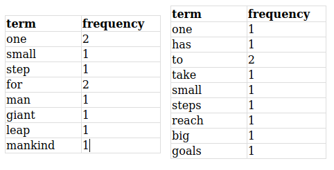
To calculate the tf-idf of "one", we first calculate its tf which is the raw-frequency. thus tf of "one" is:
$$ tf("one", Doc1) = \frac{2}{10} = \frac{1}{5} = 0.2$$ $$ tf("one", Doc2) = \frac{1}{10} = 0.1$$ The idf of a term is constant for the entire corpus and is calculated as the logarithm of total number of documents in corpus divided by the number of documents that contains the term. Thus, the idf for term "one" is: $$ idf("one", {Doc1,Doc2}) = log(\frac{2}{2}) = 0$$ Since tf-idf is defined as: $$ tf-idf_{(t,d)}= (1+log_{10}tf) * \log_{10} \frac{N}{df_t} $$ we get $$ tf-idf_{("one",Doc1)}= (1+log_{10}0.2) * 0 = 0 $$ $$ tf-idf_{("one",Doc2)}= (1+log_{10}0.1) * 0 = 0 $$ Since the t-idf is zero for the word "one", ... it means that this word is not very informative and appears in all the documents.
Let's calculate the tf-idf for another word "to". The tf of "to" is: $$ tf("to", Doc1) = \frac{0}{10} = 0 $$ $$ tf("to", Doc2) = \frac{2}{10} = 0.2 $$ The idf for term "to" is: $$ idf("to", {Doc1,Doc2}) = log(\frac{2}{1}) = 0.301$$ The tf-idf for "to" is: $$ tf-idf_{("to",Doc1)}= (1+log_{10}0) * 0.301 = 0 $$ $$ tf-idf_{("to",Doc2)}= (1+log_{10}0.2) * 0.301 = 0.30 * .30 = 0.09 $$ The word "to" is more interesting as it occurs twice in the second document.
Here we have taken (1+log 0) to be 0, since log 0 is undefined and we want to have weight as 0 when the term is not present.
To calculate the tf-idf score for the entire document, one can just sum up the tf-idf scores for all the individual terms.

Hubs and Authorities- HITS Algorithm

September 20, 2020

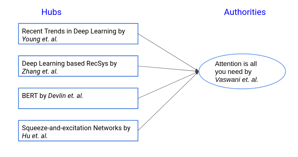
Imagine you are developing a search engine for a digital library such as IEEE Explore or arxiv and a user submits a query - What is attention ?

If you have worked in NLP or machine learning you might have heard of this mechanism called Attention introduced by Vaswani et al, in his ground-breaking research paper- Attention is all you need-  NeurIPS 2017. It was such an important concept that it changed the course of Neural Machine Translation (and of NLP ) and led to neural architecture such as Transformers, and Bidirectional Transformers(BERT) etc. See this blog post by Jay Alammar for an amazing explaination on how attention works.

Now if you make a simple text based search on all the papers in the library, you will get like million documents containing the term "attention" as it's such a common word. If you make a tf-idf based search then the original paper by Vaswani will get even lower score than the review paper by  Galassi as the former have used the term attention only 97 times as opposed to the latter who have used it more than 400 times. 

So the question is: how to figure out who is the authentic source of this mechanism called Attention? It turns out that in this network structure of linked environment i.e. if paper A cites paper B then it can be deemed as a link from paper A to paper B, one can use PageRank or HITS algorithm. HITS algorithm was developed by Prof. Jon Kleinberg at Cornell University at the same time when PageRank was developed by Larry and Sergey at Stanford. Let's see how how HITS works.

Hyperlink-induced Topic Search (HITS) is an approach to discover the authoritative sources in context of World Wide Web (www) where the number of pages is enormous and is linked to each other by hyperlinks (incoming and outgoing). But this approach could also be used for the linked structure discussed above. 

Authorative sources mean the sources which provide valuable information on the subject and has been considered as the "authority" by others due to its virtue of originality or popularity. For example, for a query on "Texas A&M University", the homepage of Texas A&M can be considered as the authority.  Pages of goverment websites might also be considered as the authorities for the query. These are the pages truly relevant to the given query and are expected by the users from the search engine.

However, there is another category of the pages called hubs, whose role is to advertise the authoritative pages i.e. they contain links to "authority" pages and help the search engine move in the right direction. For example, "usnews.com" and "timeshighereducation.com" - the sites that ranks the schools can be considered as hubs. 

Thus,

• A good hub page for a topic points to many authorative pages on that topic.
• A good authority page for a topic is pointed to by many good hubs for that topic.

For the query- "what is attention", we would have a network graph like this:

The idea behind HITS algorithm is to find out the good hubs and authorities for a topic by assigning two numbers to a page: hub score and authority score. To start with something, we first do a regular keyword search for the topic and call the search result as root set. Typically, it consists of 200 to 1000 nodes. 

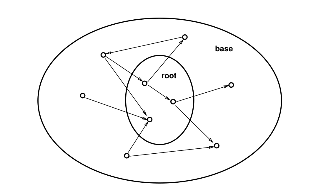
Fig1. Root set consists of examples from original query while base set consists of root set + incoming and outgoing links

Then we find all the nodes that are either pointed by the root set or points to the root set. This we call as base set( it includes the root set). Typically, it consists of around 5000 nodes. 

Next we do the following:

1. For each page x in the base set:
2. Initiliaze x: hub(x) := 1 and auth(x) := 1
3. Repeat the following update until convergence:
   • hub(x) := ∑ auth(x')  (where x' is pointed by x)
   • auth(x) = ∑ hub(x')   (where x' points to x)
   • Scale down or normalize the hub(x) and auth(x) by l2 norm (square root of sum of squares)
   
   
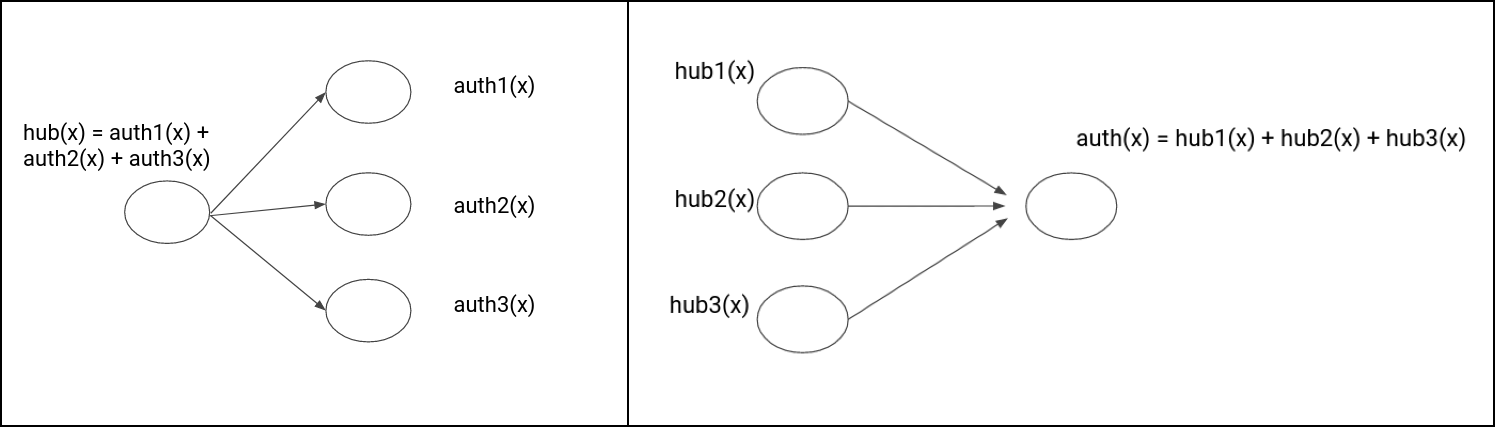
4. After convergence, the pages with highest hub scores will be the top hubs while the page with highest auth scores will be the top authorities.

Let us take a small example to understand how it works:

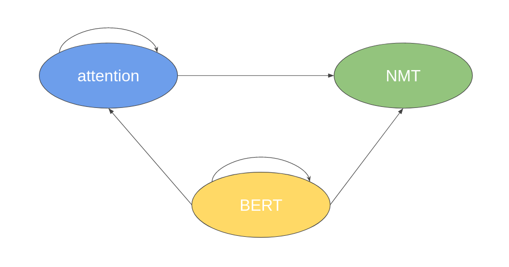
Fig2. Linked structure graph. We assign A to represent attention, B to represent BERT and N to represent NMT in the following example.

Round 0: Initialize

Hubs score	Auth score
hub (A) = 1	auth (A) = 1
hub (B) = 1	auth (B) = 1
hub (N) = 1	auth (N) = 1

Round 1:

First let's calculate the hubs score.

Since A points to A itself and N, we add the authority score of A and N from previous round to get the new_hub score for A which is = 1 + 1 = 2.

Since B points to A, B and N, we add the authority score of A, B, and N from previous round to get the new_hub score for B which is = 1 + 1 + 1 = 3.

Since N does not point anywhere,  we have the new_hub score for N which is = 0.

The l2 norm for new_hub will be = √(2^2 + 3^2 + 0^ 2) = 3.60

Dividing each element of new_hub score, we have new hubs score as follows:

Hubs Score

hub (A) = 0.55

hub (B) = 0.83

hub (N) = 0.0

Let's us now calculate the authority score.

Since A is pointed to by A and B, we add the hubs score of A and B from previous round to get the new_auth score for A which is = 2

Since B is pointed to by B, we add the hubs score of B from previous round to get the new_auth score for B which is = 1

 As N is pointed to by A and B both, we add the hubs score of A and B from previous round to get the new_auth score for N which is = 2

The l2 norm for new_auth will be = √(2^2 + 1^2 + 2^ 2) = 3

Dividing each element of new_hub score, we have new auths score as follows:

Auth Score

auth (A) = 0.67

auth (B) = 0.33

auth (N) = 0.67

Thus round 1 end can be summarized as follows:

Hubs score	Auth score
hub (A) = 0.55	auth (A) = 0.67
hub (B) = 0.83	auth (B) = 0.33
hub (N) = 0.0	auth (N) = 0.67

Round 2: 

Similar to the previous round, we will calculate first the hubs score and then authority score.

Since A points to A and N, we add the authority score of A and N from previous round to get the new _hub score for A which is = 0.67 + 0.67 = 1.34

Since B points to A,B and N, the new_hub score for B  = 0.67 + 0.33 + 0.67 = 1.67

As N does not point to anything, the new_hub score for N = 0

The l2 norm for new_hub is: √(1.34^2 +1.67^2 + 0) = 2.14

Dividing each element of new_hub score, we have new hub score as follows:

Hub Score

hub (A) = 0.63

hub (B) = 0.78

hub (N) = 0.0

Since A is pointed to by A and B, we add the hubs score of A and B from previous round to get the new_auth score for A which is = 0.55 + 0.83 = 1.38

Since B is pointed to by B , the new_auth score for B  = 0.83

As N is pointed to by A and B, the new_auth score for N = 0.55 + 0.83 = 1.38

The l2 norm for new_auth is: √(1.38^2 +0.83^2 + 1.38^2) = 2.12

Dividing each element of new_auth score, we have new auth score as follows:

Hub Score

auth (A) = 0.65

auth (B) = 0.39

auth (N) = 0.65

Thus round 2 end can be summarized as follows:

Hubs score	Auth score
hub (A) = 0.63	auth (A) = 0.65
hub (B) = 0.78	auth (B) = 0.39
hub (N) = 0.0	auth (N) = 0.65

Round 3 Calculating in a similar manner we have,

Hubs score	Auth score
hub (A) = 0.61	auth (A) = 0.66
hub (B) = 0.79	auth (B) = 0.36
hub (N) = 0.0	auth (N) = 0.66

Round 4

Hubs score	Auth score
hub (A) = 0.62	auth (A) = 0.66
hub (B) = 0.79	auth (B) = 0.37
hub (N) = 0.0	auth (N) = 0.66

Round 5

Hubs score	Auth score
hub (A) = 0.62	auth (A) = 0.66
hub (B) = 0.79	auth (B) = 0.37
hub (N) = 0.0	auth (N) = 0.66

We can see that after Round 4 there is no change in the values of hub and authority score and thus they have converged.

Page with highest hub score: BERT

Page with highest authority score(s): attention and NMT

The python code could be found here: hits.py
References-
1. Authoritative sources in a hyperlinked environment-Jon Kleinberg
2. Cornell